CFD Modelling of a Low Speed Laminar Flow
A study of flow past an equilateral triangle at low Reynolds number
Summary
In this article, I am exploring the possibilities of finding the coefficient of drag of an equilateral triangle at three different Reynolds numbers (Re) ranging from 2–30, after plotting the velocity and pressure profiles for each Re. They were then instructed to compare the results from the simulations to empirical data. A flow which is viscous and incompressible is simulated over the triangular object placed in the middle of the horizontal channel. Streamliners and Pressure fields at various Reynolds number were used to analyze the characteristics of the flow. It is found that most of the plots obtained were similar to those of the reference document provided. The article also covers the convection of air and blockages on the triangular structures at particularly specific Reynolds number.
Introduction
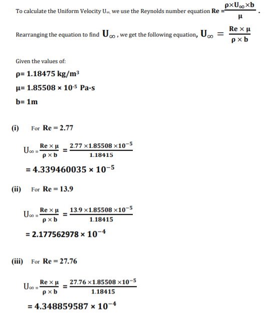
Fluid analysis is one of the most important aspects of Fluid mechanics when it comes to industrial level. Having multiple obstacles in the fluid flow path can be catastrophic for flow and can change the characteristics of flow. Hence it is very important to recognize these and to analyze the characteristics of the flow. This report is based on the analysis from the software STAR CCM+ for Computational Fluid Dynamics. The experiment is based on the flow of Air over an Equilateral Triangle obstacle placed in the middle of a horizontal wall like channel. The assessment was based on plotting velocity and pressure profiles, and the coefficient of drag of the air flow. The set of Reynolds number chosen were 2.77, 13.9, and 27.76 which lie within the given range of 2–30, and it shares the exact values as those calculated on the reference report, which allows the comparison of the results gathered. The equation for finding Reynolds number is defined by Re = 𝛒×𝐔∞×𝐛 𝛍 , where ρ is density of fluid, U∞ is uniform velocity of fluid and μ is fluid viscosity and b is the vertical side of triangular cylinder.

Method
For the most part the steps listed (adapted to the given geometry) in the “Defining Boundary Surfaces”, page 7958, and “Steady Flow: Backward Facing Step”, page 8416, were followed. These are available on the software user guide [1], details for the key sections can be seen below:
Geometry
1. Open Geometry > right click > New
2. Rename ‘3D-CAD Model 1’ to ‘Equilateral Triangle Obstacle’
3. Features > right click > XY Plane > Create Sketch. Create geometry as seen on Figure 1.
4. Sketch 1 > right click > Extrude > select 1m as the Distance. Click ‘OK’.
5. Rename the Faces of shape, by right clicking on the face > Edit, set the name and Click ‘OK’ the faces should be named, Inlet, Outlet, Top Wall, Bottom Wall, Front Wall, Back Wall, according to their position with respect to the Triangle. Also, the three Faces of the Triangle must be named as one Face, this can be achieved by rotating the view around the circle and selecting the three faces while pressing the ‘Ctrl’ key on the keyboard, and right click > Edit.
6. Right click on the front plane with largest area > Create Sketch > On Face. Plot the geometry as seen on Figure 2. Special attention must be taken to coincide the triangle of this sketch with the one on Sketch 1.
7. Sketch 2 > Extrude > Method: Up to Face, Direction Type: Reverse, Body Interaction: None Click ‘OK’.
8. Expand Body Groups Folder, rename ‘Body 1’ to ‘Tunnel’, and ‘Body 2’ to ‘Refinement Box’.


Mesh
1. Click on Simulation, expand Geometry > 3D-CAD Models > right click on ‘Equilateral Triangle Obstacle’ > New Geometry Part > Click ‘OK’.
2. Right click on Geometry > Operations, click New > Mesh > Badge for 2D Meshing. Select ‘Tunnel’ from Parts list, click OK.
3. Right click ‘Badge for 2D Meshing’ and click ‘Execute’.
4. Right click on Parts > Tunnel, and click Assign Parts to Regions.
5. Select ‘Create a Region for Each Part’ and ‘Create a Boundary for Each Part Surface, ‘Apply’ and ‘Close’
6. Expand Regions > Tunnel > Boundaries > Inlet, and set ‘Type’ to ‘Velocity Inlet’. Also select the type for Outlet, as ‘Pressure Outlet’.
7. Right click Geometry > Operations and select New > Mesh >Automated Mesh. Select ‘Tunnel’ and select ‘Surface Meshers’ as ‘Surface Remesher’ and ‘Core Volume Meshers’ as ‘Trimmed Cell Mesher’. Click OK.
8. Click Automated Mesh > Meshers > Trimmed Cell Mesher, activate ‘Perform Mesh Alignment’
9. On Automated Mesh> Default. Set on ‘Base Size’ the value as 0.2m, on Minimum Surface Size > Percentage of Base as 100, and ‘Mesh Alignment Location’ as [0.0, 1.0, 0.0] m.
10. Right click Operations > Automated Mesh > Custom Controls, and select New > Volumetric Control. Select Volumetric Control > Parts Property as ‘Refinement Box’.
11. Expand Volumetric Controls > Controls > Trimmer, and activate ‘Customise isotropic size’ option on the ‘Properties’ section. Then open Values > Custom Size and on ‘Properties’ select ‘Percentage of Base’ to 50.0.
12. Click on the ‘Generate Volume Mesh’ bottom on the top bar. When it finishes running right click on Scenes folder, New Scene > Mesh, the image seen should be the same as that on Figure 3.

Physics
1. Right click Continua > Physics 1 > Models, click on ‘Select Models’.
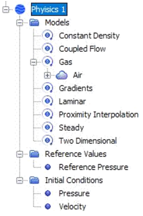
2. Select on ‘Time’, Steady. ‘Material’, Gas. ‘Flow’, Coupled Flow. ‘Equation of State’, Constant Density. ‘Viscous Regime’, Laminar. The ‘Physics 1’ should look like on Figure 4. Pressure on Reference Values > Reference Pressure and on Initial Conditions > Velocity should be set to zero.
3. Right click on the Reports folder, New Report > Force Coefficient.
4. On ‘Force Coefficient 1’ set the Reference Density as that on Continua > Physics 1 > Gas > Air > Density > Constant. On the ‘Parts’ section select Tunnel > Equilateral Triangle.
Extracting Numerical Solutions
The calculated velocity for each Reynolds number must be set with the same value at three locations:
1. Continua > Physics 1 > Initial Conditions > Velocity, ‘Value’ under ‘Properties’ section, the first value of the matrix been modified and the second one left at zero.
2. Regions > Tunnel > Inlet > Physics Values > Velocity, just as on the first location, the ‘Value’ section and only the first number of the matrix.
3. Reports > Force Coefficient 1 > Reference Velocity.
Calculations
Screenshots
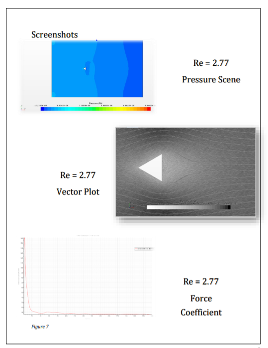
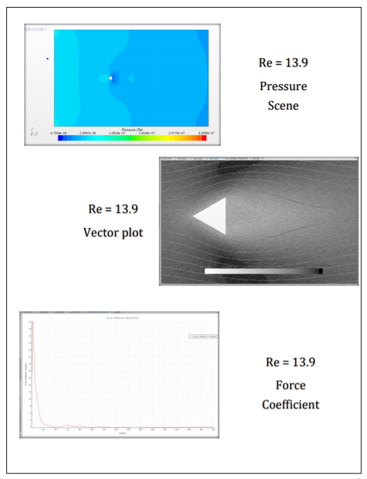
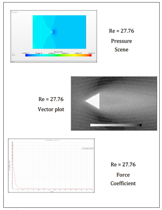
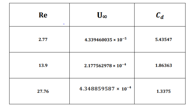
Table of Data
Data for the Coefficient of Drag (𝐶𝑑) was extracted from the 300th y-value of the respective Force-coefficient graph of each Reynolds Number.
Data Analysis
After gathering all the necessary data, it can be seen that those for the respective Re values share great similarity in the shapes of the vectors and streamlines formed.
It can be observed that the Drag Coefficient (𝐶𝑑) decreases exponentially in the collected data with a comparable trend to that of the given Cd against Re graph, seen in Figure 8

Discussion of errors
The stopping criteria for this experiment was set at 300, if a larger number had been selected, the accuracy of the Coefficient of Drag would have increased getting closer to that of the given Cd against Re graph.
Conclusion
From the above experiment it can be concluded that the laminar viscous flow over an Equilateral triangle obstacle is investigated by the particular Finite volume scheme. The simulations run for a set of 3 different Reynolds numbers, within the range of 2–30 with respect to the empirical data that shows a similar amount of drag acting on the triangle. Velocity vectors show that, for very low Reynolds number, flows are symmetric and there are variations in the results of the drag. Using a numerical method it can show different results. The streamlines and flow parameters such as the drag coefficient are found. It is noticeable that with an increase in the Reynolds number, the flow will continue to remain symmetric, but during the formation of eddies the symmetric flow region decreases and change to the asymmetric region. Accordingly the drag coefficients on the equilateral triangle decreases with increase in the Reynolds number in symmetric regions.
Bibliography
[1] Siemens PLM Software, Simcenter STAR-CCM+® Documentation, SIEMENS, 2019.
[2] R. S. e. al, “Assessment of Air Flow over an Equilateral Triangular Obstacle in a horizontal Channel Using FVM,” Journal of Mathematical Sciences and Applications, 2013.